15. Hough Transform to Find Lane Lines
title
Implementing a Hough Transform on Edge Detected Image
Now you know how the Hough Transform works, but to accomplish the task of finding lane lines, we need to specify some parameters to say what kind of lines we want to detect (i.e., long lines, short lines, bendy lines, dashed lines, etc.).
To do this, we'll be using an OpenCV function called
HoughLinesP
that takes several parameters. Let's code it up and find the lane lines in the image we detected edges in with the Canny function (for a look at coding up a Hough Transform from scratch, check
this
out.) .
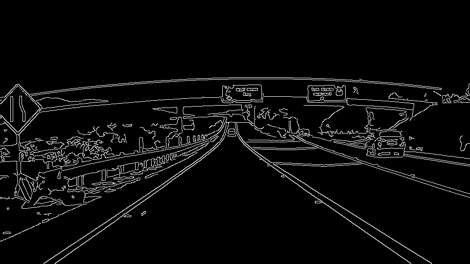
Here's the image we're working with:
edges_exit
title
Let's look at the input parameters for the OpenCV function
HoughLinesP
that we will use to find lines in the image. You will call it like this:
lines = cv2.HoughLinesP(masked_edges, rho, theta, threshold, np.array([]),
                                             min_line_length, max_line_gap)
In this case, we are operating on the image
masked_edges
(the output from
Canny
) and the output from
HoughLinesP
will be
lines
, which will simply be an array containing the endpoints (x
1
, y
1
, x
2
, y
2
) of all line segments detected by the transform operation. The other parameters define just what kind of line segments we're looking for.
First off,
rho
and
theta
are the distance and angular resolution of our grid in Hough space. Remember that, in Hough space, we have a grid laid out along the (Θ, ρ) axis. You need to specify
rho
in units of pixels and
theta
in units of radians.
So, what are reasonable values? Well, rho takes a minimum value of 1, and a reasonable starting place for theta is 1 degree (pi/180 in radians). Scale these values up to be more flexible in your definition of what constitutes a line.
The
threshold
parameter specifies the minimum number of votes (intersections in a given grid cell) a candidate line needs to have to make it into the output. The empty
np.array([])
is just a placeholder, no need to change it.
min_line_length
is the minimum length of a line (in pixels) that you will accept in the output, and
max_line_gap
is the maximum distance (again, in pixels) between segments that you will allow to be connected into a single line. You can then iterate through your output
lines
and draw them onto the image to see what you got!
So, here's what its going to look like:
# Do relevant imports
import matplotlib.pyplot as plt
import matplotlib.image as mpimg
import numpy as np
import cv2

# Read in and grayscale the image
image = mpimg.imread('exit-ramp.jpg')
gray = cv2.cvtColor(image,cv2.COLOR_RGB2GRAY)

# Define a kernel size and apply Gaussian smoothing
kernel_size = 5
blur_gray = cv2.GaussianBlur(gray,(kernel_size, kernel_size),0)

# Define our parameters for Canny and apply
low_threshold = 50
high_threshold = 150
masked_edges = cv2.Canny(blur_gray, low_threshold, high_threshold)

# Define the Hough transform parameters
# Make a blank the same size as our image to draw on
rho = 1
theta = np.pi/180
threshold = 1
min_line_length = 10
max_line_gap = 1
line_image = np.copy(image)*0 #creating a blank to draw lines on

# Run Hough on edge detected image
lines = cv2.HoughLinesP(masked_edges, rho, theta, threshold, np.array([]),
                            min_line_length, max_line_gap)

# Iterate over the output "lines" and draw lines on the blank
for line in lines:
    for x1,y1,x2,y2 in line:
        cv2.line(line_image,(x1,y1),(x2,y2),(255,0,0),10)

# Create a "color" binary image to combine with line image
color_edges = np.dstack((masked_edges, masked_edges, masked_edges))

# Draw the lines on the edge image
combo = cv2.addWeighted(color_edges, 0.8, line_image, 1, 0)
plt.imshow(combo)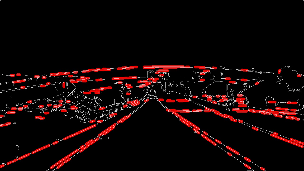
hough_text_outro
As you can see I've detected lots of line segments! Your job, in the next exercise, is to figure out which parameters do the best job of optimizing the detection of the lane lines. Then, you'll want to apply a region of interest mask to filter out detected line segments in other areas of the image. Earlier in this lesson you used a triangular region mask, but this time you'll get a chance to use a quadrilateral region mask using the
cv2.fillPoly()
function (keep in mind though, you could use this same method to mask an arbitrarily complex polygon region). When you're finished you'll be ready to apply the skills you've learned to do the project at the end of this lesson.